Robot Control System for 3D Concrete Printing Based on an Open PLC. We frequently find industrial six-axis robotic arms or gantry robots in industrial applications connected to 3D concrete printing technology, the employment of which may not be totally appropriate for this technology. The kinematic structure of the aforementioned robots is typically not directly optimized for 3D concrete printing applications, and they are typically equipped with closed control systems that do not provide complete control flexibility to users.
The goal of this article is to introduce and evaluate the open control system platform of a one-of-a-kind robot for 3D printing buildings. Because of the industrial control system employed, this platform provides for easy integration into the industrial process while still being accessible enough for educational and research reasons. The installation of model-based control of the experimental model of the printing robot, which serves as a test bed for the final version of the printing robot, demonstrates the system’s openness.
Printing Robots
Control Systems for Printing Robots
Gantry robots were among the earliest robots employed in the application of 3D concrete printing. The primary reason for this is because gantry robots are very straightforward to manage and can carry big weights. A cost-effective solution for the mechanical and control system of a gantry robot is detailed, allowing the printing of a free curved structure constructed of fiber-reinforced mortar without the use of a mold. The gantry robot is made up of three-axis linear actuators attached to a box-like support structure. According to the needs of each axis, linear actuators are realized by a belt or a ball screw. Brushless DC servo motors with gearboxes power the individual actuators. The useful print area measures 1300 mm 950 mm 800 mm, with the x-axis being the longest and operated by two synchronous motors in tandem for greater mechanical load capability.
The x- and y-axes have maximum speeds of 500 mm/s, while the z-axis has a maximum speed of 300 mm/s. An integrated Personal Computer (PC) with a PC/104 interface transmits positioning instructions to the individual servocontrollers through a Controller Area Network (CAN). In terms of software, the control PC runs a G-code interpreter that calculates the position trajectory at a maximum frequency of 500 Hz and then transmits real-time commands to the subcontrollers.
Matlab is used by the control system to simulate the trajectory in order to check the position trajectory and prevent system faults. According to the authors, the advantage of their solution lies in the distributed control system, which aims at cost reduction, flexibility, scalability, and deployability for a variety of applications, including the construction of atypical structures and unattended construction in hazardous locations.
Six-axis industrial robots were used in 3D concrete printing a bit later than gantry robots, but they allowed for the manufacturing of far more geometrically complicated items. Six-axis industrial robots are much more difficult to handle than gantry robots, but they have more flexibility of movement and take up less space.
The Open Robot Control System Based on PLCs
The standard industrial PLC/PC from Bernecker + Rainer Industrial Automation (B&R) firm (B&R Industrial Automation GmbH, Eggelsberg, Austria) serves as the foundation for the open control system for the printing robot. The openness of this system is made possible by the use of a “automatic code generator.” Control models from the Matlab/Simulink environment are transformed by the automated code generator into C/C++ programming code that may be automatically executed on the PLC [33].
With the help of common function blocks and libraries, also known as mapp components, and the ability to use more complex control techniques in the Matlab/Simulink environment, we are able to construct software.
In Figure 1.1, a human-machine interface (HMI) and an open PLC-based control system for a printing robot are shown. PLK stands for an Ethernet powerlink bus, SDL for a shielded data link connector, and HMI for shielded data link connector.
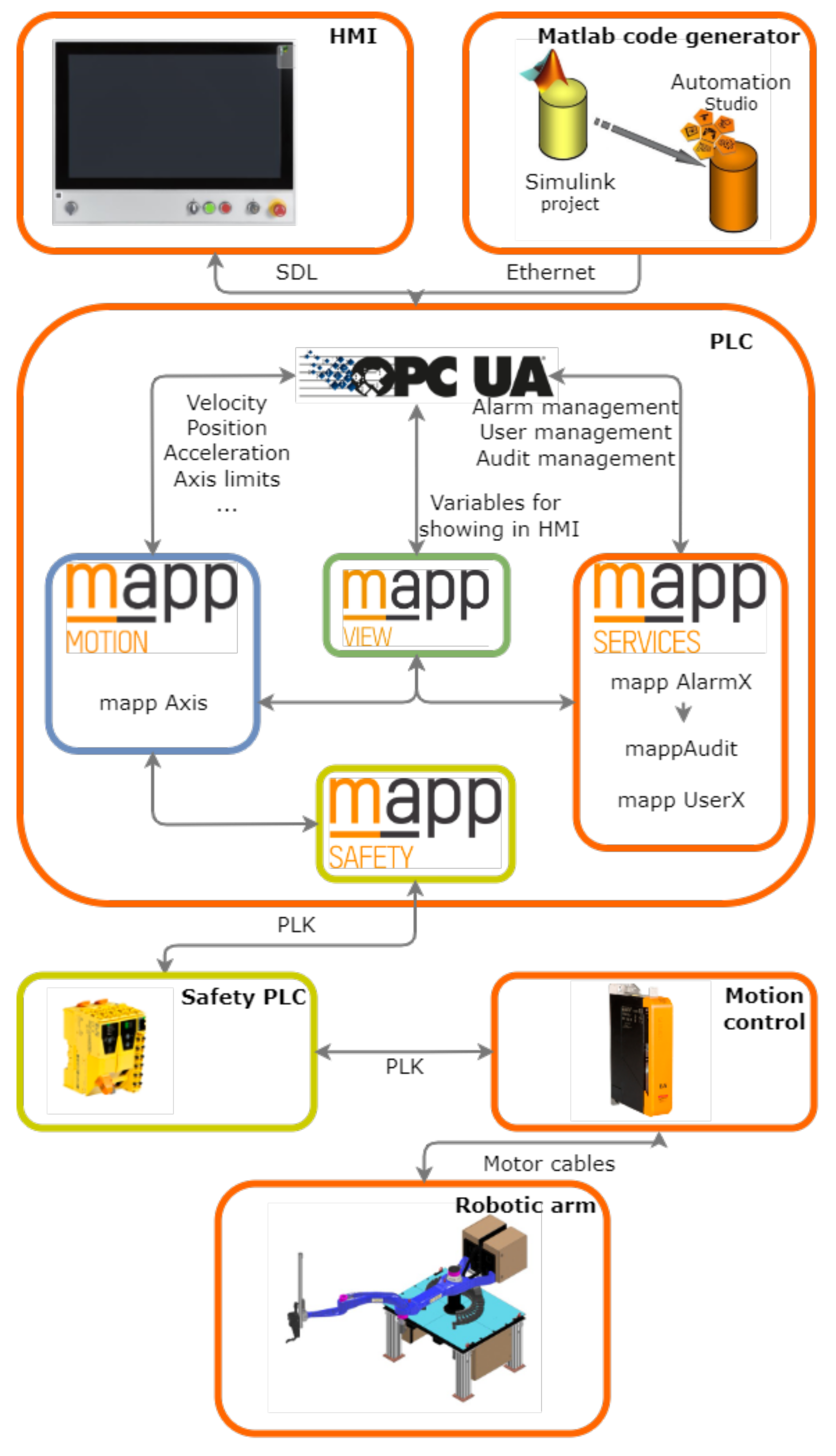
Figure 1.1 depicts a printing robot with an open control system based on a PLC.
Software
The robotic arm’s software consists of four layers: mapp-mapp motion, mapp services, mapp vision, and mapp safety. Figure 1 depicts a block layout with layers. From the perspective of a programmer, the maps provide functional blocks, functions, and configuration files to facilitate software development. They then give the machine operator with an intuitive interactive environment that allows the machine to be controlled more easily. The page contains further information on how to use the mapp components (mapp Motion, mapp View, and mapp Services). Furthermore, mapp Safety is employed in the control system to assure the printing robot’s safety.
Mapp Safety integrates safety technologies completely into the mapp framework, making it easier to design, manage, and troubleshoot safety applications. If the publicly accessible user’s human-machine interface (HMI) application is insufficient to meet the needs of the customer application, a standard mapp interface allows for the implementation of more complicated functionalities.
Processes of the Basic Control System
One of the fundamental functions of robotic manipulator software has always been to perform four fundamental processes that allow robot integration into an automation system: motion trajectory generation and tracking, motion/process integration and sequencing, human-machine interface, and information integration.
- Motion Trajectory Generation and Tracking: The range of manipulation that can be programmed, as well as the capacity to accomplish controlled programmed motion utilizing real-time control at the servo level, are important features of motion generation for robotic manipulators. Mapp Motion components are used for trajectory development and motion tracking, in conjunction with an automatically produced job provided by Matlab/Simulink, which manages time and motion interpolation.
- Motion/Process Integration: Coordinating the motion of the manipulator with process sensors or other devices is what this procedure is all about. The most basic process integration occurs via digital inputs/outputs (I/O) or their readout via the control PLC. Mapp Safety handles a little more advanced error-free process integration. Technology mapp Safety enables the project to quickly adopt safety standards. The application is isolated from other applications and operates on a customized safety PLC with independent operation. The primary goal of mapp Safety is to keep users safe. It responds to the TOTAL stop button by turning off the activation control on the Acapus inverter and stopping the machine.
- Human Integration: The controller’s human-machine interfaces are critical to its functioning, allowing for the efficient setup and control of robotic systems. This interface is managed by mapp View. The visualization gets information about the Open Platform Communications United Architecture (OPC UA) server’s activated function blocks and variables. Multi-client and multi-user access solves the problem of personalized content. The apps may be seen on mobiles, tablets, laptops, or any device that has a web browser. The last HW generation robotic arm employs a TFT touch automation panel with a 54.64 cm diagonal big screen and a metal bar holding control components. The application consists of five pages: the main page, the table page, the alert page, the audit page, and the service page (all restrictions and parameters). The primary page is the most significant page for the control arm. This website includes three forms of robotic arm control: basic positioning, tool center point (TCP) mode, and trajectory mode.
- Information Integration: According to the standards for Industry 4.0, one of the most important features of a machine is information. There are several forms of information, such as machine, user, and programmed information. Mapp Services technology is utilized for information integration, and the Audit function allows users to retain user, machine, and program data in user memory or view it in a graph. The saved data might be utilized for machine maintenance or operator inspections. A screen from an industrial camera, for example, can be utilized as an information source in a visualization application.
G-Code Interpreter
There are two versions of the G-code interpreter algorithm. The first option is a user solution, in which the user simply uploads (through a USB flash drive, for example) a 3D model of the printed object converted to G-code format. The control system then handles time-based coding and sequential movement of the robot’s print head while taking kinematic limitations into consideration, utilizing the Interpreter configuration file contained with mapp Motion. In this scenario, the effective locations of the robot joints are determined using mapp Motion’s unique mechanical system component. Using a configuration file, this component enables the creation of a non-standard mechanical system. In our situation, we built five configurations with unique inverse kinematics solutions, and the user may select the desired version based on the needs of the printed product.
The second approach is a research solution in which G-code translation is handled by a custom G-code interpreter written in Matlab and the inverse kinematics problem is handled by an autonomously generated task written in Matlab/Simulink. This technique enables us to have far more comprehensive control over the arm, as well as the capacity to tune its motion.
The desired print head position path and material application speed are obtained in both cases using special software that converts the CAD model of the printed object in STL format into a G-code containing the endpoint coordinates and parameters for the temporal parameterisation of the motion path. We will utilize the program StarSlicer developed by our team or the commercially available software Grasshopper for this purpose. Figure 1.2 shows two different versions of the G-code interpreter.

Figure 1.2 shows a G-code interpreter.
Torque Control at the Lowest Level
To implement more complex control techniques (model-based approaches), it was essential to address the implementation of torque control, ideally real-time torque control, in addition to the traditional position/velocity servo control. According to the PLCopen standard, the fundamental function blocks for position and velocity control (MC_MoveAbsolute, MC_MoveRelative, and MC_MoveVelocity) are provided for standardised motion control.
For conventional torque control applications (e.g., winding applications, etc.), the standardised function block MC_TorqueControl is utilized. This function block, however, is inappropriate for our application since it does not support cyclic torque input and has a speed constraint. The difficulty of cycling the torque and bypassing the speed limitation that results in speed saturation when the motor is lightened has to be solved for the robotic arm’s real-time torque management capabilities.
Different approaches to addressing these torque control needs were investigated, and the following technique was successfully implemented to achieve cyclic torque input in the absence of speed limits.
Figure 1.3 depicts the final solution of the real-time torque control option. This technique entails removing the cascaded servo control structure’s speed and position controller and then cyclically programming the appropriate parameter identifier (Par Id) with the necessary torque to the Acopos servo amplifier. The whole control is managed by a Matlab/Simulink model that gives the time of the cyclic input. During testing, the approach performed admirably and proved to be a success.

Figure 1.3: PLC torque control.
Hardware
During the first phase of the open control system’s development, a so-called zero generation robotic platform was created, which consisted of a simplified 1:4 scale replica of a printing robot that served as a test bed and was controlled by a simplified control system known as Zero HW generation. The Zero HW generation used a reduced power B&R PLC 5APC2100 with an Acopos invertor and three axes with synchronous servo motors and planet gears. Arm control has been addressed through the use of an easy visualization that can be accessed via any device that has a web browser.
A first-generation robotic platform was created during the second phase of the open control system’s development. This robotic platform has a 1:2 scale printing robot in relation to the final printing robot, which is operated by the same control system as the final printing robot, thus the designation final HW generation. The last HW generation improved the hardware configuration. B&R’s powerful PLC 5PC910.SX02, synchronous motors with precise harmonic gears, a Safety PLC, an HMI display, and a sturdy aluminum structure were utilized.
The first-generation robotic platform contains a printing robot that satisfies the specifications for an industrial robotic arm capable of carrying the 3D printing head and producing the structure. The zero-generation robotic platform is used to evaluate the open control system before it is deployed on the first-generation robotic platform and the final printing robot.
Figure 1.4 depicts the distinct HW setups of the robotic platforms.

Figure 4: Comparison of HW configurations
Zero Generation Robotic Platform Modelling
As indicated in the preceding section, a simpler experimental arm and control system, dubbed the zero-generation robotic platform, were created for preliminary testing.
This reduced control system operates on the same principles as the final control system for the printing robot. The acquired results should thus be simply transferrable to the final control system and the 1:2 scale printing robot, both of which are now being commissioned and tested.
On the zero generation robotic platform, the capabilities of the proposed open control system was first analysed and confirmed. The overall goal of verifying the openness of the proposed control system is to show model-based control implementation.
To do this, a kinematic and dynamic model of the robot under test must be developed first. The kinematic characteristics of the printing robot’s simplified model provide the equations of motion determined using the Euler-Lagrange technique. Finally, there is a set of minimal inertial parameters known as basis inertial parameters, in which the equations of motion may be stated and recast into a linear relationship.
Printing Robot Simplified Model and Kinematic Model
A reduced 1:4 scale replica of the printing robot’s experimental model was built for testing the open control system. It is a redundant planar robot with 3DOF achieved by three articulated steel plate linkages. Figure 1.5 depicts the printing robot model’s kinematic structure and kinematic parameters.
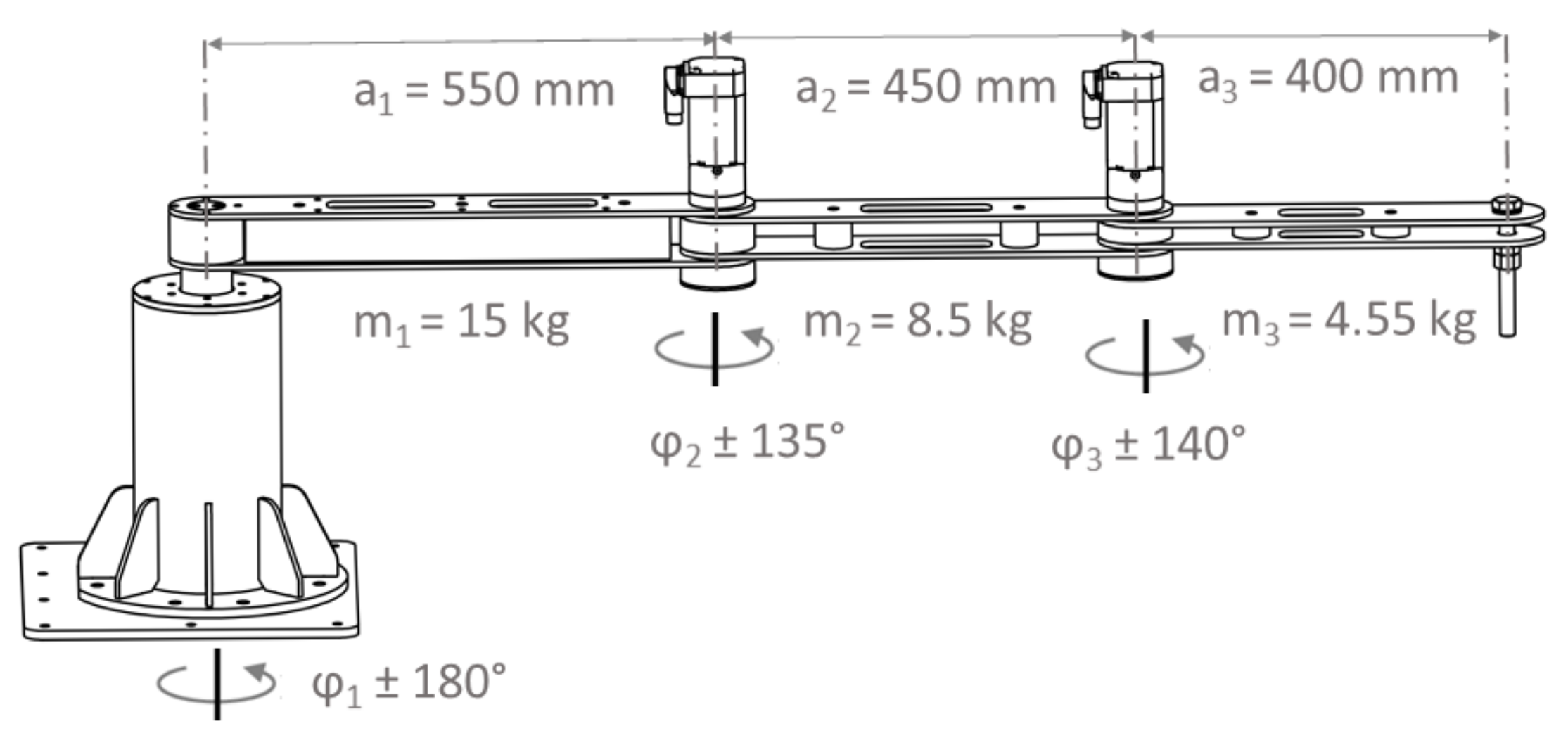
Figure 1.5 shows the simplified model of the printing robot’s kinematic framework.
It is fairly simple to solve the direct kinematics issue; the transformation equations for the arm terminal coordinates are as follows.
𝑥=𝑎1 cos𝑞1 + 𝑎2 cos(𝑞1+𝑞2) + 𝑎3 cos(𝑞1+𝑞2+𝑞3)
𝑦=𝑎1 sin𝑞1 + 𝑎2 sin(𝑞1+𝑞2) + 𝑎3 sin(𝑞1+𝑞2+𝑞3)
𝑞𝑗,min≤𝑞𝑗≤𝑞𝑗,max, 𝑗=1,2,3
The joint angles must be entered and the appropriate x and y coordinates must be calculated in order to solve the direct problem. The inverse kinematics problem is substantially more challenging and sophisticated to solve. The related Jacobi matrix is of type 23 and has no inverse representation since the robot manipulator has redundant degrees of freedom. In the context of the inverse robotics problem, the issue entails calculating the angles q1, q2, and q3 for a given point with x, y coordinates by solving a single system of equations:
- Using one of the angles as a parameter, compute the other angles;
- To arrive to the following equation, choose a fixed constraint between the angles q1, q2, and q3.
- As an extremal issue for the selected optimization criterion, determine the angles q1, q2, and q3.
The first two choices are acceptable for locating the inverse problem’s analytical solution. By selecting the various angles as variables, the first solution choice offers three other options. It makes sense to take into account a linear restriction that leads to the other two solution alternatives for simplicity and practical applications. The second solution option introduces a constraint that, in general, may be applied in any number of ways.
The whole derivation of the inverse problem of the kinematics of a printing robot is covered. The inverse issue is converted to the complex plane in this case, and exponential functions are used to solve it.
This post covers the comprehensive derivation of the inverse problem of a printing robot’s kinematics. In this step, the inverse problem is converted to the complex plane and solved using exponential functions. All five possibilities for the analytical solution of the inverse kinematics issue are derived in this study.
Simplified Printing Robot Dynamic Model
The robot dynamics were calculated using a rigid body model derived from the Euler-Lagrange formulation. The following equation may be used to define the dynamic model of the robot manipulator with friction:
𝐌(𝐪)𝐪¨+𝐂(𝐪,𝐪˙)𝐪˙+𝐛(𝐪˙)+𝐠(𝐪)=𝞽
where 𝐪,𝐪˙,𝐪¨∈ℝ𝑛 , 𝐌(𝐪) is an (𝑛×𝑛) inertia/mass matrix of the robotic manipulator, which is symmetric and positive definite, 𝐂(𝐪,𝐪˙) is an (𝑛×𝑛) matrix of Coriolis and centrifugal forces, and 𝐛(𝐪˙) is an (𝑛×1) vector of friction forces, which is most often represented by the viscous and Coulomb friction components:
𝐛(𝐪˙)=𝐅𝐯𝐪˙+𝐅𝐜sgn(𝐪˙)
where 𝐅𝑣 and 𝐅𝑐 are (𝑛×𝑛) diagonal matrices with coefficients corresponding to individual joints. Furthermore, 𝐠(𝐪)∈ℝ𝑛 is the gravity vector and 𝞽 is an (𝑛×1) vector of generalized forces/torques.
Inertial Base Parameters
In Section 4.2, a dynamic model of the robot was created using Lagrange’s equations, which contain the typical nonlinear functions 𝐪,𝐪˙,𝐪¨ and standard dynamic parameters that occur in the matrix of moments of inertia of the i-th component of the robotic arm:
𝐉𝑖=⎡⎣⎢⎢⎢⎢⎢⎢⎢−𝐼𝑥𝑥𝑖+𝐼𝑦𝑦𝑖+𝐼𝑧𝑧𝑖2𝐼𝑥𝑦𝑖𝐼𝑥𝑧𝑖𝑚𝑖𝑥̲𝑖𝐼𝑥𝑦𝑖𝐼𝑥𝑥𝑖−𝐼𝑦𝑦𝑖+𝐼𝑧𝑧𝑖2𝐼𝑦𝑧𝑖𝑚𝑖𝑦̲𝑖𝐼𝑥𝑧𝑖𝐼𝑥𝑦𝑖𝐼𝑥𝑥𝑖+𝐼𝑦𝑦𝑖−𝐼𝑧𝑧𝑖2𝑚𝑖𝑧̲𝑖𝑚𝑖𝑥̲𝑖𝑚𝑖𝑦̲𝑖𝑚𝑖𝑧̲𝑖𝑚𝑖⎤⎦⎥⎥⎥⎥⎥⎥⎥𝑖=1,2…𝑛
where Ixxi,Iyyi, and Izzi are main moments, Ixyi,Ixzi, and Iyzi are products of inertia of link i, xi, yi, and zi are the coordinates of the centre of gravity, and m are masses with respect to the i-th link frame, respectively.
Let us divide the common dynamic parameters into two vectors. 𝐩𝑑∈ℝ10𝑛×1 is a vector composed of masses, inertial parameters, and the Cartesian position of the mass center of the robot’s linkages. where 𝐩𝑓∈ℝ2𝑛 is a vector containing the friction properties of the robot’s joints, as shown below:
𝐩𝑑,𝑖𝐩𝑓,𝑖=[𝐼𝑥𝑥𝑖,𝐼𝑥𝑦𝑖,𝐼𝑥𝑧𝑖,𝐼𝑦𝑦𝑖,𝐼𝑦𝑧𝑖,𝐼𝑧𝑧𝑖,𝑚𝑖𝑥̲𝑖,𝑚𝑖𝑦̲𝑖,𝑚𝑖𝑧̲𝑖,𝑚𝑖]𝑇=[𝐹𝑐𝑖,𝐹𝑣𝑖]𝑇
It is always feasible to recast the robot dynamic model (1) in a linear form with regard to the standard dynamic parameters using the regressor matrix Y, which depends solely on the kinematic variables.
𝐘(𝐪,𝐪˙,𝐪¨)𝞹(𝐩𝑑,𝐩𝑓)=𝞽
where the vector
𝞹(𝐩𝑑,𝐩𝑓)=(𝐩𝑇𝑑𝐩𝑇𝑓)𝑇∈ℝ𝑝.
A number of conventional dynamic parameters do not play a role in the dynamic model of a specific robot, as the relevant columns of the regressor matrix are zero. Some standard settings may only be displayed as fixed. The regressor matrix’s associated columns are linearly dependent. We may isolate 𝑏≪10𝑛 independent sets of parameters and divide the matrix Y into two parts, with the second group comprising the dependent (or zero) columns as 𝐘dep=𝐘indep𝐓 for the corresponding constants 𝑏×(10𝑛−𝑏) of matrix 𝐓.
𝐘(𝐪,𝐪˙,𝐪¨)𝞹=(𝐘indep𝐘dep)(𝞹indep𝞹dep)=
(𝐘indep𝐘indep𝐓)(𝞹indep𝞹dep)
=𝐘indep(𝞹indep+𝐓𝞹dep)=𝐘(𝐪,𝐪˙,𝐪¨)𝐚
The dynamic coefficients can be derived heuristically by rearranging and combining the separate dynamic parameters; guidelines for getting the dynamic coefficients based on the robotic manipulator’s kinematic structure are provided. Numerical approaches such as SVD (singular value decomposition) or QR decomposition can also be used to calculate dynamic coefficients. Due to the minimal number of degrees of freedom in our scenario, the basic inertia values were computed heuristically.
Experiment Design for Testing the Zero Generation Robotic Platform
To show the control system’s openness, an experiment was constructed to cover all of the processes required to deploy model-based control.
First, in the Matlab/Simulink environment, a kinematic and dynamic model of a scaled printing robot was developed using Equations (1)-(3). These models were validated by comparing them to models generated by the Matlab Robotic System Toolbox. The dynamic model of the robot was recast in linear form with regard to the base standard parameters (see Equation (7)), and the base inertia parameters were chosen heuristically with respect to the regressor matrix’s complete rank.
Following that, we designed an experiment for parametric identification of robot inertia parameters by moving the robot along a specially designed identification trajectory (also known as an excitation trajectory) and then measuring the torque of individual robot links.
The identification experiment was designed primarily to select a suitable excitation trajectory that provided enough excitation of the robot dynamics to manifest all dynamic parameters and thus achieve a fast and accurate estimation of these parameters even in the presence of disturbances. A trajectory consists of the sum of harmonic functions that is periodic and band limited for possible trajectory optimization and additional signal processing.
Each axis’s joint trajectory may be expressed as a finite Fourier series of the sum of harmonics:
𝑞𝑗(𝑡)=∑𝑙=1𝐿𝑎𝑙,𝑗𝑙ω𝑓sin(𝑙ω𝑓𝑡)−𝑏𝑙,𝑗𝑙ω𝑓cos(𝑙ω𝑓𝑡)+𝑞0,𝑗
where L is the number of harmonics chosen, ω𝑓 is the signal frequency chosen, and the coefficients 𝑞0,𝑗, 𝑎𝑙,𝑗, and𝑏𝑙,𝑗 may be computed using the optimization technique.
It is easier to acquire the excitation trajectory for robot identification by solving an optimization issue because least squares methods demonstrate that the condition number of the regressor matrix Y must be reduced to decrease the influence of noise in the calculations.
In Matlab/Simulink, the excitation trajectory parameters were improved using the fmincon function (nonlinear minimization with constraints) and the SQP (sequential quadratic programming) technique. To ensure the highest numerical stability for the following least squares parameter estimate, an objective function that minimizes the condition number of the regressor matrix was used.
The motion constraints selected here limit the joint locations, velocities, and accelerations, as well as the position of the robot’s end effector in Cartesian space. These limitations are selected to respect the physical capabilities of the robot actuators while preventing collisions between the robot and objects in its surroundings (when a forward kinematics problem is considered).
A dynamic model of the robot was built based on the acquired inertia parameters, and we then designed a control-based model to govern the scaled model of the printing robot. The traditional feed-forward control in the form of inverse dynamics compensation (FFW) + PD control was adopted for the purposes of this work.
𝐮=𝐮̂𝑑+𝐊𝑃(𝐪𝑑−𝐪)+𝐊𝐷(𝐪˙𝑑−𝐪˙)
where Kp and KD are the position and velocity gains (or damping), which are often diagonal. The feed-forward component supplies the needed joint forces for the desired manipulator state (𝐪,𝐪˙,𝐪¨) , while the feedback term adjusts for any mistakes caused by uncertainty in the inertial parameters, unmodeled forces, or external disturbances.
Experiment Findings
The experimental setup comprises of a printing robot experimental model (shown in Figure 1.6) and a prototype open PLC-based control system. The excitation trajectory was created and refined in the Matlab/Simulink environment to determine the inertia parameters, as shown in Equation (10). The optimization of the excitation trajectory parameters resulted in the condition number of the regressor matrix being reduced to 2.8. Figure [1.7] depicts the excitation trajectories for the printing robot experimental model after solving the optimization issue, using ω𝑓=0.15×𝞹 and 𝑡∈[0,21], in addition to L = 5.

Figure 1.6: shows Printing robot experimental model.

Figure 1.7: shows Excitation paths that have been optimized.
The excitation trajectory was then implemented in an open control system using an automated code generator, with each joint controlled in “trajectory control mode” via decentralized control accomplished via cascade control of the control system’s servo amplifier. During this action, joint torque signals were captured at a sample time of 400 μs. The basic inertial parameters were then computed and compared with the inertial parameters derived from the 3D model of the printing robot’s experimental model using Autodesk Inventor. To compare the observed and reconstructed torques, the robotic arm was moved along a separate excitation route and the torques on each axis were recorded.
Figure 1.8 depicts a comparison of the observed joint torques with the torques calculated from the indicated parameters using Equation (7), where 𝑢1 , 𝑢2 , and 𝑢3 directly correspond to the torques on the separate actuators of the robotic arm.
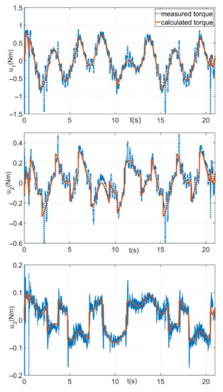
Figure 1.8 shows the difference between estimated and measured torques.
Table 1 displays the identification results, the symbolic representation of the individual base inertia parameters, and a comparison of the identification parameters to those acquired from the 3D model.

Table 1 shows the base inertia parameters that were found and derived from the 3D model.
If we regard the model’s parameters to represent the real parameters of the arm, the highest percentage error in parameter estimate is less than 28%, which is not the best outcome. However, because the 3D model has limited precision and the impact of, for example, supply cables, etc., on the arm, the assumption of accepting the inertia of the parameters acquired from the 3D model as the real ones is not particularly significant in practice. The torque traces comparing the estimated and real torques show that the torques derived from the specified factors represent the observed torques quite well.
The experiment concluded with the installation of the control based on the acquired dynamic model. The reference trajectory was generated using a fifth-order polynomial in joint space. The motion of all joints was based on zero, with the first axis moving from (0∘,45∘,0∘) at a peak velocity of 53.71∘/𝑠 and a peak acceleration of 105.3∘/𝑠2, and the second and third axes moving from (0∘,±90∘,0∘) at a peak velocity of 107.43∘/𝑠 and a peak acceleration of 210.6∘/𝑠2. The resultant motion corresponds to the “folding” and “unfolding” of the robotic manipulator, and the trajectory was created only for test control reasons, with the axes interacting. The intended trajectories for each joint are shown in Figure 1.9.
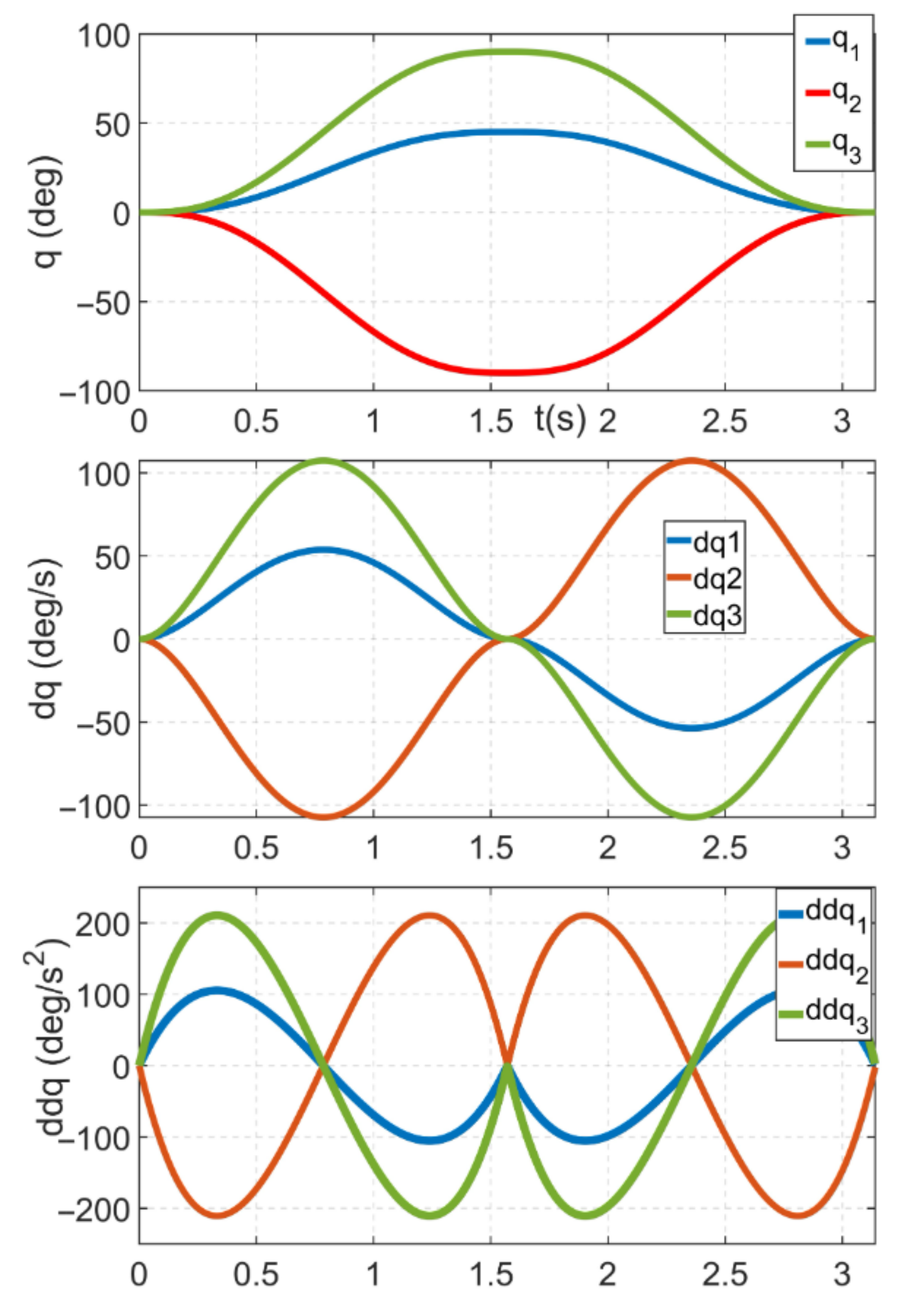
Figure 1.9 illustrates the desired fifth-order polynomial trajectories.
To compare the control outcomes based on the dynamic model developed, the arm was initially controlled via decentralised cascade control, as in the identification experiment, and the control deviation at each joint was measured. The cascade control’s individual loops were initially adjusted using the control system manufacturer’s default autotuning process. Table 2 shows the individual controller gains acquired by the autotuning technique.

Table 2 shows the cascade controller parameters for individual joints.
Following that, the suggested feed-forward control was performed, with an action intervention in the form of a desired torque being cyclically created with a period of 400 μs.
Based on the dynamic model, Figure 10 compares the trajectory inaccuracy between the decentralised control and the implemented feed-forward control. The feed-forward controller considerably decreased the trajectory errors for joints 2 and 3, with peak errors of just 0.36∘ and 0.2271∘, respectively. The tracking errors were comparable for joint 1, although the feed-forward controller had a lower control action.
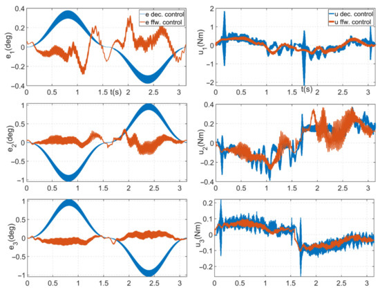
Figure 1.10 depicts the two controllers’ trajectory tracking faults and associated control actions.
Robotic Platform of the First Generation
When compared to the zero generation platform, the first generation of the robotic platform was upgraded with a variety of components, peripherals, and functionalities. The platform was built to allow testing of both the printing and important components for fully automated printing such as localization, self-leveling, and printing robot calibration, as well as the ability to deploy advanced control methods to obtain the greatest possible printing accuracy. The platform is now being deployed and tested on a 1:2 scale experimental print arm in comparison to the final print arm.
Printing Experiment Arm
The experimental print arm has the same kinematic structure as the final print arm and is based on the SCARA framework with an extra rotating axis. The arm has four degrees of freedom, as shown in Figure 1.11, and its kinematic structure consists of three sequential rotating axes (a1-a3) and a final translational axis (a4). The arm’s length is 2.8 m, the endpoint’s vertical stroke is 1 m, and the maximum load on the endpoint is 35 kg. Individual arm members were created using generative design to provide optimum stiffness at a low weight and are manufactured of aluminum alloy utilizing CNC chip cutting technology.
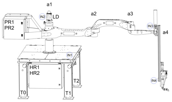
Figure 1.11: A view of the Printing Mantis with inclinometer sensors.
The Printing Robot’s Final Control System
The first-generation robotic platform’s whole control system is a distributed control system separated into four control cabinets (HR1, HR2, PR1, and PR2) that are networked via the POWERLINK industrial bus (PLK). The robotic platform is powered by a total of eight drives: four for the print arm and four for the robotic base. The control components for the various drives are housed in the separate enclosures. B&R synchronous servo motors control the translational axes, ensuring extremely accurate placement. To provide a chatter-free connection, the arm rotary axes are controlled by high-end synchronous servo motors with harmonic gears from Harmonics Drive.
Extruder and tangential axis drives are also available for expansion. The printing compound—a cement mixture—will be extruded from the print head via the extruder axis. The tangential axis offers an extra alternative axis for turning the print nozzle in order to rotate it in the direction of nozzle movement in order to test different nozzle shapes.
As previously stated in subchapter Section 3.5, the control system incorporates a very powerful control PC and four servo drivers capable of controlling up to 12 axes, with the servo driver for rotary axis control being enhanced with SafeMotion capabilities based on openSafety technology.
This technology enables the activation of integrated safety measures such as safe speed limits to provide maximum safety for the print robot operator. The control system is supplemented with a big and robust HMI for controlling the robot platform.
Added Peripherals
The control system is built with novel peripherals like as tilt meters and lidar to test the self-leveling of the robot base and tackle print arm localization issues. To compensate for unevenness and deviations from the print plane, the experimental print arm is outfitted with four Sick inclinometers. The primary inclinometer, marked IN1, is positioned in the robot table plane, as shown in Figure 1.11. It measures tilt along three axes (x, y, and z) and may be used to level the table with the surroundings. The remaining inclinometers, denoted by the letters IN2, IN3, and IN4, are situated directly on the robot arm assembly.
IN2 and IN3 are inclinometers that can measure tilt in two x,y axes. They are used to monitor any deflection of the lidar (LD) and the arm’s end link (a3). The last inclinometer, IN4, is tri-axial as well and is designed for the case of expanding the robot with a tangential axis; its output can provide information on the rotation of the tangential axis on which a print head can be mounted. Another peripheral is a SICK 2D lidar, model SICK NAV350 (SICK AG, Baden-Wuerttemberg, Germany). Endpoint localization and guiding capabilities are provided by LD lidar in this application.
First Generation Robotic Platform Commissioning and Testing, as well as Printing Concepts
The first generation robotic platform is being commissioned and tested right now. Before 3D printing systems can be deployed, a variety of activities must be completed, such as robotic arm calibration, tuning of individual actuator controllers to remove endpoint vibration, testing of localization principles, and so on.
The robot was outfitted with an Ortur 10W LU2-10A laser module (Ortur Intelligent Technologies Co., Ltd, Dongguan, China) used in engraving machines in order to track the endpoint of the print arm along the required print trajectory.
The module employs dual-compression diode technology, which is based on the interference of two laser diodes’ light beams. This solution allows you to evaluate the repeatability and precision of the robot’s endpoint, as well as monitor the endpoint’s vibration, which is plainly evident in the “engraved waveforms.” With this technology, we may consider all parameters when developing new control algorithms for the robotic arm. Figure 1.12 shows a video of the testing, in which the robot “engraves” one of the experimental print paths in the shape of an 800 x 400 mm experimental wall element.
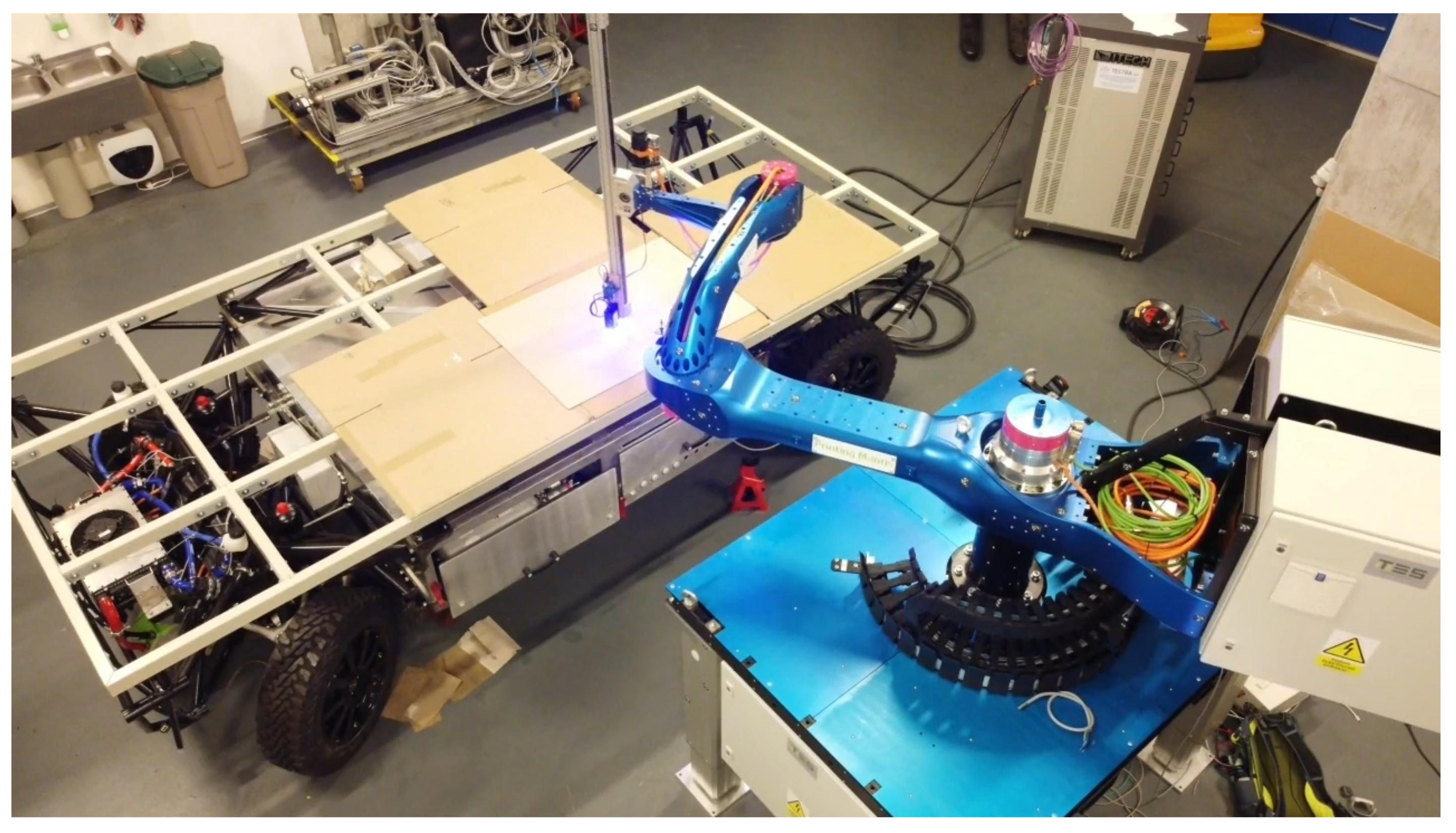
Figure 1.12: Experimenting with a printing robot
The robotic arm is intended for a sequential printing application, in which the printing robot travels about the site and prints building structures, or sections of building structures, successively inside its workspace. The crane or the robot’s own mobile platform can be used to move it. The primary challenge in completely automating the sequential printing process is locating the printing equipment on the job site, which will be accomplished using the aforementioned lidar.
The robot prints in individual layers dictated by the printing medium and in steps determined by the printing height of the object to be printed. The last movement axis of the robot is responsible for changing the print head height by one printed layer. When the robot reaches the maximum printing height of one step, the extension columns elevate the robot base by a predetermined distance, allowing the robot to print the next layer. An electronic shaft engages the drives of the extensible columns of the robotic base between the parts for synchronized movement and to keep the robotic base horizontal.
Individual legs can be positioned separately at the start of printing to adjust for surface abnormalities. Because of the inclinometers employed, this stage may be completed automatically, with the robot base automatically levelled. Figure 1.13 shows a video of a robot base lift test in which the robot base is lifted by a defined test height of 1800 mm.

Figure 13: Lifting the experimental printing robot’s robotic base
I absolutely loove your blog and find nearly all of our post’s to be just what I’m looking for.
Does one offer guest writers to write content available for you?
I wouldn’t mind writing a post or elaborating on some off thhe subjects
you write in relation to here. Again, awesome site! https://www.waste-Ndc.pro/community/profile/tressa79906983/
Thank you.