Design of Lightweight Robots

Design of Low-Cost Lightweight Robots Using Computational Systems

Current industrial robots make automation more cost-effective by delivering consistent performance for high-volume manufacturing over lengthy durations. However, as the trend towards mass customization continues, specialist industrial robots are frequently acquired and set up for low-volume procedures, rising the overall cost of operation. Furthermore, traditional industrial robots are large and unsuitable for human-in-the-loop tasks.

Modular robots, on the other hand, can adapt to changing user demands, making them a viable alternative to fixed architecture robots. Furthermore, reconfigurability opens up the possibility of realizing non-intuitive kinematic structures by covering a large design space with a diverse set of interchangeable robot configurations. [6] investigates the design of cost-effective modules and standardized interfaces, whereas [7] presents a model of human safety in the presence of reconfigurable robots. However, such robots inherit traits from ordinary industrial robots such as high gear ratio joints, solid metal bodies, and so on, increasing their weight, cost, and complexity. Modular robotic kits, on the other hand (Robot modules from Keyi robotics), provide a simple and user-friendly interface for building robots.

The current study provides a computational design technique based on interdisciplinary design optimization [8] to bridge the gap between industrial and residential robots in order to produce low-cost, lightweight robots on demand. To implement such robot manipulators, the planned 3D printed modules include joints, connections, and end-effectors that physically and electrically link with one another. Furthermore, as illustrated in Figure 1, their interface design allows for the creation of physically practical robots. In contrast to traditional structural optimization techniques that include static loads, the topology optimization issue in this study accounts for dynamic loads caused by the robots’ mobility to build lightweight yet suitably stiff structural components.

 

 

 

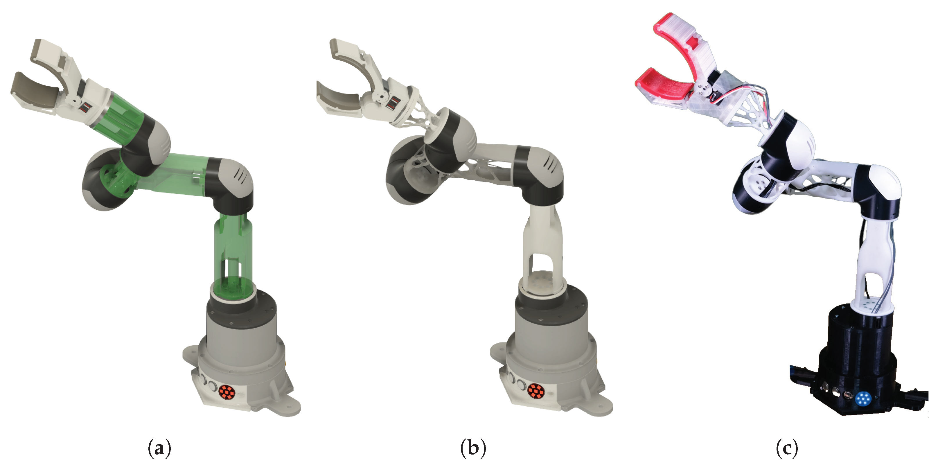
Figure 2.1. The robot in (a) is the result of an autonomous design technique that determines a workable architecture utilizing modules. The structural components are not optimized at this point, and the space coloured in green represents the accessible domain for topology optimization. The components of the robot in (b) are optimized structural elements (OSEs) after the component optimization process. Finally, all of the components are 3D printed and combined to create a physical prototype of the robot depicted in (c), (as seen in the Supplementary Materials).

While several strategies for identifying task-specific robot compositions have been presented, a few challenges remain, including the physical feasibility of the simulation results, i.e., sim-to-real transfer of the identified robot, and resolving the circular dependency between the robot configuration and mass optimal design of modules under dynamic loading. The present effort intends to bridge the gap between the design of robot systems and component-level structural optimization. The following are the primary contributions of this work:

Designing Task-Specific Robots Automatically

Previously, [12,14] explored the development of robot morphology and related controls for a certain job. [24,25] explored the optimization of continuous design factors such as link length, actuator performance, and so on for a fixed robot architecture. Furthermore, the work given in [26,27] investigates methods for exploring the design space using preset modules that meet desired task criteria. Design abstractions are required to construct meaningful robots when working with a discrete set of heterogeneous modules, as outlined in [28,29]. To tackle the combinatorial complexity involved with the challenge of determining the right sequence of the modules, methods such as informed search in [30], reinforcement learning in [31], genetic algorithms in [26], and graph heuristic search in [32] were examined.

 

Furthermore, [33] described the automated development of equations of motion for a particular robot design. [34] investigates the co-design of modular tensegrity structures, whereas [35] investigates the evolution of modular robots without inter-modular communication. Furthermore, numerous evolutionary techniques for design space exploration have been examined, such as the use of novelty search and local competition outlined in [36] and compositional pattern-producing networks depicted in [37]. [7] stresses the need of automated safe programming of modular robots in human-centric situations. [6] proved the value of autonomous development of hardware and communication interfaces in reducing the time necessary to deploy a reconfigured robot in an industrial scenario. The present study takes a similar approach while underlining the need of designing modules that permit physical feasibility, or guarantee the actual reality of a particular robot configuration.

 

[50] offered a concept for decoupling a multi-component system based on the so-called solution space, allowing the independent design of the individual components. In [51,52], a meta-model-informed decomposition was presented, which eliminated the requirement for coordination between sub-problems. The current study uses a distributed optimisation technique to calculate mass optimum topologies of robotic linkages by dissecting system-level needs into component-level specifications.

 

 

 

Figure 2 depicts the design process in the form of an extended design structure matrix (XDSM [57]). Table 1 shows the definitions of the linked input-output variables for each design stage. Each green rectangle represents a design process, while the grey channels reflect the flow of information. The white parallelograms represent the outputs of one step, while the grey parallelograms represent the inputs to the next step. Furthermore, the black arrows indicate the direction and sequencing of the steps.

 

 

 

An explicit statement of the system’s higher-level needs is a critical component of the strategy. In Figure 2, these criteria are incorporated into the design process and establish the permissible ranges of the QoIs. To illustrate the operation of the proposed computational systems design method, for example, a robot design meeting the requirements given in Table 2 must be identified. The specifications correspond to a typical pick and place application in which the robot’s end-effector is expected to transport a 1 kilogram payload between the specified beginning and ending places. Using bottom-up and top-down mappings, the top-down design method seeks to find component-level requirements necessary to create such a robot.

Table 2 shows the system-wide multidisciplinary requirements.

 

 

Figure 3: Modules: (a) Passive OSE modules with green design domain sections enabling fastener assembly and cable routing. The interfaces that connect the OSEs to the other modules are shown by the grey borders. (b) The passive connections, which were left out of the topology optimisation. (c) The motors are housed in an actuated joint module. (d) The electronics and microcontroller are housed in the base module. (e) A module with end-effectors.

Several practical design decisions have also been made to make the assembling process easier. All of the modules are assembled with conventional M3 screws, and the fastener orientation, size, and torque strength provide secure and dependable connections. This not only informs the OSE’s design domain, but it also specifies the print orientation of the appropriate OSEs so that the embedded nuts can withstand the loads when fastened. In addition, the design allows for the construction of a joint module to an OSE in 10 minutes and the entire assembly of a five-degree-of-freedom robot in 2 hours. This allows for faster troubleshooting and reduces robot downtime.

However, when dealing with computationally complex sensors (such as pictures or point cloud inputs) or situations involving costly decision-making stages (online planning or MPC), more powerful control hardware may be required. While off-the-shelf solutions are convenient and inexpensive for prototyping, as the number of modules grows, bespoke PCBs may become economically viable. They provide for more design flexibility and quick replacement of electrical components in times of scarcity.

Compositions C(M) and Connection Rules c

When combining the components to create robots, not all combinations provide meaningful results. As explained in [28], connection rules serve as the foundation for the algorithm in identifying physically possible combinations and guiding the design process with module semantic information. Connecting the outputs of two joint modules, for example, would essentially create no meaningful output torque. To capture only relevant module combinations, a set of connection rules that regulate the interaction between the modules is developed. As a result, the created robot assemblages, known as compositions, are meaningful and physically realizable. In this context, the terms composition, robot composition, and architecture can all be used interchangeably.

min𝐶(𝑀),𝐾𝑐∑𝐼,𝐺(𝑔𝑝𝑎𝑡ℎ(𝐶(𝑀))+ℎ(𝐶(𝑀))),

subject to,𝒑𝑒𝑒𝑓(0)=𝒑𝐼,𝒑˙𝑒𝑒𝑓=𝟎,

𝑔(𝒒(𝑡),𝒒˙(𝑡))≤0,

𝑔𝑔𝑜𝑎𝑙(𝒒(𝑇),𝒒˙(𝑇),𝒑𝐺)≤0,

𝐶(𝑀)∈𝐶𝑝(𝑀,𝑐),

where 𝒒(·)∈ℚ is the robot’s setup. Inequality constraints 𝑔(·) (1c) are used to enforce limits on joint angles, velocities, torques, and the allowed ranges of the QoIs. (1c) additionally includes inequality restrictions that limit the minimum distance between any two bodies while accounting for probable self and environmental collisions. The cost function f() for the optimization issue is defined as the sum of the route cost, 𝑔𝑝𝑎𝑡ℎ(·), and the heuristic cost, ℎ(·). The cost function 𝑓(·) is assessed at both the beginning and final end-effector locations 𝒑𝐼,𝒑𝐺, while the total completion time restriction is employed to modify the control DVs, Kp, and Kd.

 

Figure 5: An example exhibiting the ability to discover a suitable robot composition capable of overcoming obstacles inside the workspace (represented as collision limitations by grey cylinders and spherical geometric primitives).

 

Alternatively, the problem can be changed to one of feasibility by setting the cost function f=0, resulting in a constraint fulfilment problem [62,63]. Instead of a single solution, a group of solutions that fulfil the stated conditions may be discovered by creating so-called solution spaces, as shown in [50,55]. It is not, however, immediately relevant in the current example, which involves a mixed combination of continuous and discrete DVs. The current technique may easily be expanded to find a family of suitable compositions by continuing the search until all compositions matching the conditions are located.

where s is the length of the ith OSE, mp is the payload mass (1 kg), and g=9.81ms2 is the gravitational acceleration. The decomposition shown in Equation (3) allows for the breakdown of system-level needs to the component level while maintaining system-level performance. Furthermore, such a decomposition enables the independent optimization of specific OSEs, effectively parallelizing the optimization sub-problems.

ℱ𝑐(𝑖),𝑗=ℱ(𝑖)(𝑡𝑐(𝑖),𝑗),where𝑗=1…6,

𝑡𝑐(𝑖),𝑗=argmax𝑡ℱ(𝑖),𝑗(𝑡),

where ℱ𝑐(𝑖),𝑗 is a 6-dimensional vector carrying the jth critical load situation for the ith component. The goal of the ith OSE structural optimization is to decrease its mass while not exceeding the component-level critical compliance determined from Equation (3) for all j critical load instances.

min𝜌𝑒(𝑥)     𝑚(𝑖)(𝜌𝑒(𝑥))

such that      𝑙(𝑖)≤𝑙𝑐(𝑖),

for load cases    ℱ𝑐(𝑖),𝑗,and𝑗=1…6,

where 𝑚(𝑖),𝑙(𝑖) are the mass and compliance energy of the ith OSE, respectively, and e represents the elemental density field over the ith OSE’s possible design domain Ω. Following the technique would result in four distinct topology optimization sub-problems defined by Equation (6). Each sub-problem of topology optimization, optimizes the elemental density field 𝜌𝑒 over the design domain depicted in Figure 3. Furthermore, each sub-problem is subjected to distinct critical compliances 𝑙𝑐(𝑖) and loads obtained from Equations (3) and (5), resulting in distinct topologies for each of the OSEs, as shown in Figure 7.

The controller employed in the current study to actuate the hardware prototype is also made accessible in Section 8’s data availability declaration.

It should be noted that the identified task-specific robot has four degrees of freedom and thus costs less for the number of actuators used than similar commonly deployed standard robots (for example, the commercially available MyCobot Pro 600 from Elephant robotics) with six or seven degrees of freedom. This is due to the designed robot focusing solely on the essential task. However, such a comparison should be made, with the distinction that the latter is a general-purpose robot, whilst the former is a task-specific robot.

 

 

 

Figure 8 depicts the simulated mobility of the robot with the post-processed modules between the required places, as well as the corresponding joint torques achieved.

As smaller-scale fixed-base robots are industrial scale robots, the difference in advantages may not be considerable [65]. To comprehend their applicability to various contexts, a full research of such components’ scalability and related expenses must be done.

Physical Prototype Construction and Testing

The OSEs were 3D printed for the physical prototype using Form labs’ Rigid 10K (the Rigid 10k material from Form labs) resin (https://formlabs.com/, last viewed on 16 June 2023). Figure 1c depicts a prototype of the manufactured post-processed modules. Finally, the built robot was assessed in relation to the requirements listed in Table 2. The actual robot’s recorded mobility time between the indicated places is 4.5 s, which is near to the mandated limit value. Furthermore, the robot’s end-effector deflection under 1 kg force is evaluated.

The first stance of the robot is chosen for testing since the load conditions (Figure 6) are for the specified motion beginning with this pose. Figure 9 depicts the test setup for end-effector deflection. The measured deflection of the end-effector is about 11 mm, which deviates from the specifications. Although the observed structural deflection of the OSEs is relatively small and may be within the derived component-level compliance energy, it is important to note that a significant portion of the end-effector deflection can be attributed to the joints’ unaccounted structural stiffness.